GEOG 6000 Advanced Geographical Data Analysis
Analyzing Social, Economic and Political Factors that Impact Environmental Sustainability through Principal Component Analysis
Abstract
Creating a sustainable environment has long been an important issue for individuals and political entities. A recent WalletHub article put together a report of the relative performance of each state in the US based on their environmental policy, pollution rates and consumption of basic resources. While this provides a measure of environmental friendliness, it does not explain what creates the milieu that drives this behavior. Using another set of criteria not specifically related to environmental sustainability, social, political and economic factors will be examined that influence a state’s overall “green” rating. Employing a multivariate analysis approach known as principal component analysis, this study will focus on understanding the correlation between the social, economic and political factors in better environmental practices. An understanding of what makes up a community that is capable of living more sustainably could perhaps help foster or direct other communities in how to do the same.
Introduction
This year WalletHub, a financial statistics website, produced a metric for determining the most environmentally friendly and sustainable states in the US. (Kiernan, 2018) The article used three areas of impact to determine a score for a state's’ overall performance, and ranking among other states, in “green” or environmentally friendly behavior. The three areas were environmental quality, for factors such as air, water and soil quality, eco-friendly behavior, which accounted for green energy, recycling and water usage, and climate change contributions, measuring output of greenhouse gases. When the results of this analysis were used to create a map of the US with states ranked visibly by level of “greenness”, it was obvious there was a spatial pattern in the state’s relative scores. Areas such as New England, the Pacific West and the Great Lakes region had similar and higher rankings relative to other states. The Deep South, the Grain belt (Indiana, Illinois, Iowa, Kansas, Nebraska) and the Southwest states had low rankings within a similar range. This obvious geographic distribution indicates other potential underlying factors that influence a state’s approach to sustainability.

Figure 1. Map of US created with “Green” ratings from WalletHub
There are many different conditions that influence environmentally sustainable practices. In this study we will examine several social, economic and political indicators and their relationship to the results of the WalletHub study. The main method of analysis will be a type of multivariate analysis known as principal component analysis. Principal component analysis (PCA) has proved beneficial in revealing variables responsible for geographic phenomenon in previous studies (Petrisor et al., 2012). Petrisor et al. detail the results of using PCA in combination with GIS in four case studies in Romania to understand the underlying variables that influence development. In each case they found that often the development could not be explain with a single category or variables (education, economics, demographic etc), but rather was best modeled by variables from different categories. PCA has also been used to identify features of communities that are aware and supportive of green energy (Bhowmik et al. 2018). The study found certain commonalities, such as education, income, political involvement, in communities that support the use of green energy. These commonalities were subsequently identified and recommended for development in regions that are not as involved or supportive of green energy (Bhowmik et al. 2018)
Social and economic conditions have a documented role in environmental sustainability. (Lange et al. 20009, Pebley 1998, Rudra et al. 2018, Orenstein 2011, Merkel 1998, Bhowmik et al. 2018) The argument behind this is rather obvious, when individuals have a good living standard, education and access to basic necessities there is time and opportunity to focus on environmental concerns. Among the most impactful social factors are education levels, and access to healthcare or federal assistance programs for lower income groups. (Bhowmik et al. 2018, Lange et al. 2009) Economic factors with significant bearing on environmental behavior are household income, the political entity’s GDP. (Lange et al. 2009, Pebley 1998) Wealth disparity can be a tremendous factor in waste creation and huge jumps in energy consumption. In developing areas, new wealth tends to mimic consumption habits of Western nations. This can create large amounts of energy and resource consumption in regions without refined practices for reducing pollutants and handle waste responsibly (Lange et al. 2009)
Political conditions have an impact on environmental practices as well. Rudra et. al. discusses the negative impact political heterogeneity can have on a political entity’s environmental policy. Without cohesive political leadership or support, enforcement of regulations can be unreliable. (Rudra et al. 2018) Most entities face issues of variant and often divergent political groups, which can make unified legislation difficult (Orenstein et al. 2011)
Methods
The green score is the result of a study conducted by WalletHub, a financial advisement platform. The scores are potentially from 0 - 100, with the higher score resulting in a lower number rank. In the data, the lower the rank the better the state did in the scoring matrix. (Kiernan, 2018) For the PCA I used the overall score out of 100, so factors that positively correlate to the score will be an indicator of improved environmental practices.
Social variables represent the quantity of educational facilities in the state, percentage of high school graduates, and percentage of college graduates with a bachelor’s degree. Also in the social category is the percent of the unemployed labor force (temporary unemployed) that collect public healthcare. The health care percentage does not account for privately insured unemployed, which is approximately double the publicly insured percentage, or those who do not collect insurance through either private or public providers. This statistic also does not account for long term unemployed citizens who may or may not by insured by a public healthcare program.
Economic variables represent several different metrics. Orenstein et al. discuss the importance of diversified industry in the economic, and conversely environmental, health of a region. In order to create a statistic to reflect this and index was created containing the gap between the industry with the largest number of employees and the the industry with the lowest number of employees. Average median income and unemployment rates are meant to test the overall prosperity of individuals in each state, while the averaged state GDP will illustrate the economic prosperity of the state over the last ten years.
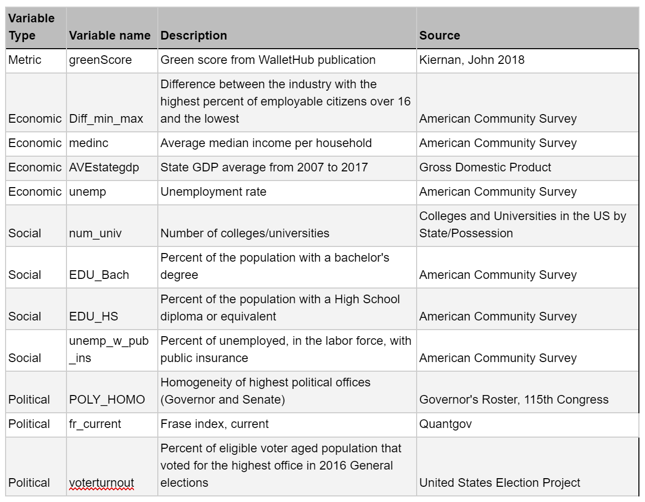
Figure 2. Variables and descriptions
Political homogeneity was created by applying a uniformity percentage to the political offices of the Governor and two Senators from each state. As these are elected officials the relative homogeneity of the state should be reflected in their parties. The FRASE Index is a weighted score applied to each state and represents the relative economic impact federal legislation has on the state. Much of the source of greenhouse gases and other pollutants is derived by industry and the private sector. The FRASE index represents the ability of the federal government to regulate industry in each region. (Quantgov) The final variable is a percentage of voter aged population who participated in the 2016 general election in minimally casting a vote for the highest office on the ballot.
Each variable was read into a single file to facilitate converting to a matrix in R. The variables were not originally in the same scale, so once the data was read in the variables were scaled. For the principal component analysis, the prcomp() function was employed, as it has been documented this approach provides more accurate results (STHDA).
Results
Initial output from the PCA indicates that the majority of the variance within the model is explained by the first through the sixth axis. Five percent is not a great increase, but the threshold for explanation in this model was 85%, so I have chosen to analyze the six principal components (PC). Review of the coefficients for each PC indicates some expected correlations. The first axis shows a positive correlation between green scores and higher levels of education, higher percentage voter turnout and higher median income. It appears the first access is capturing the positive influence of affluence in a developed nation of environmental practices.(Pebley, 1998) This access also conveys a negative correlation between the green score and the FRASE index and higher unemployment rates. The negative impact from unemployment is anticipated, as unemployment rates increase it is an indicator of other issues in the state and may make environmental policy less of a priority. The FRASE index seems to indicate the less government regulation is linked to higher green scores, however it is not entirely clear the impact of that variable.

Figure 3. Proportion of model explained by each principal component
The second axis is covering the number of universities and colleges and the state GDP. These variables both have slight negative relationships to the green score which is an interesting revelation. The four largest GDPs are California, Texas, Florida and New York. This can be seen plainly in Figure 5, the four states are outliers on this axis. New York and California both have relatively high greenscores but these are also the four most populous states and Florida and Texas both ranked relatively low in environmental quality from the WalletHub assessment. The number of universities in a state having a negative correlation seems contrary to the strong positive correlation between green score and education rates.

Figure 4. Variables plot from PCA
The third, fourth and fifth access do not seem to represent any related trend in the variables. That the political homogeneity would have a negative correlation with the variation in industry does not seem like a legitimate relationship. Other relationships are already expressed in their impact on the green score, so the fact that as unemployment escalates voter turnout decreases, while a logical conclusion, is not pertinent to this analysis.
Discussions
The spatial pattern originally spotted in the WalletHub article seems to be replicated in the biplot of the individual variables against the geographic units. The New England states with the highest green scores are grouped in the Figure 5. They have higher rates of high school and college graduation as well as higher median incomes and voter turnout. On the opposite end, the Deep South is grouped together with lower graduation rates and higher unemployment. An interesting correlation is the political homogeneity and the regions in the Grain belt and the Southeast. These states are mostly completely homogenous, with the Governor and Senators belonging to the same political party. This relationship indicates that in the US perhaps it’s policy related rather than political heterogeneity that has a relationship the the environmental sustainability of the state.

Figure 5. Plot of individual states from PCA
Several of the outlier states from the WalletHub report come into a clear image when plotted against the variables as in Figure 5. South Dakota and Colorado were both geographic anomalies, ranked fifth and twenty first respectively when the majority of their immediate neighbors were ranked in the thirties and forties. Here on this plot, South Dakota evidently has lower rates of high school and college graduation, lower median income and voter turnout and lower industry diversity than other states that ranked higher in green scores. Colorado however follows the trend of the New England and Pacific Northwest states. It seems likely that other demographic data not included in this analysis is affected South Dakota’s environmental impact.

Figure 6. US Scores from WalletHub study
Conclusions
Environmental practices are a result of the natural environment, but also how people interact with their environment. The social, economic and political variables chosen for this analysis illustrate this complex relationship between the community and the environment. Sustainable practices are not simply a result of legislation and regulation, but of the overall well being of the population. The correlation between public access to health care, education, income, involvement in politics and a diverse economy communicates what Lange et al. discussed; when a society reaches a certain level of affluence, and is no longer struggling to meet with daily necessities, there is more potential and resources to devote to creating a sustainable relationship with the environment.
While most of the states in the WalletHub report had scores within a five to ten point range, the lowest scoring states and highest scoring states had a significant point difference from the mean. For the states that ranked on the low end, West Virginia and Kentucky, it may be beneficial to understand that there is a correlation between social and economic well being of the population and their impact on the environment. Improving one could lead to improvements in environmental conditions.
References
115th Congress, https://www.senate.gov/senators/index.htm
American Community Survey, https://www.census.gov/acs/www/data/data-tables-and-tools/
Bhomik, Chiranjib, Bhomik, Sumit, Ray, Amitava. 2018. Social Acceptance of Green Energy Determinants using Principal Component Analysis. Energy 160:1030-1046.
Colleges and Universities in the United States of America By State/Possession. http://www.univsearch.com/state.php 12/06/2013.
Gross Domestic Product. https://www.bea.gov/data/gdp/gross-domestic-product. 11/28/2018.
Governors Roster 2018, Governors’’ Political Affiliations and Terms of Office. https://www.nga.org/governors-2/
Kiernan, John S. 2018’s Greenest States. https://wallethub.com/edu/greenest-states/11987/, 04/17/2018.
Lange, Willem J. de, Wise, Rusell, and Nahman, Anton. 2009. Securing a Sustainable Future Through a New Global Contract Between Rich and Poor. Sustainable Development 18: 374-384.
Merkel, Angela 1998. The Role of Science in Sustainable Development. Science 281(5375): 336-337.
Orenstein, D.E, Jiang, L., Hamburg, S.P. 2011. An Elephant in the Planning Room: Political Demography and its Influence on Sustainable Land-Use Planning in Drylands. Journal of Arid Environments 75: 596-611.
Pebley, Anne R. 1998. Demography and the Environment, Demography, 35 (4): 377-389.
Petrisor, Alexandru-Ionet, Ianos, Ioan, Iure, Daniela, Maria-Natasa Vaidianu. 2011. Applications of Principal Component Analysis Integrated with GIS. Procedia Environmental Sciences 14: 247-256.
STHDA: Principal Component Analysis in R: prcomp vs princomp, http://www.sthda.com/english/articles/31-principal-component-methods-in-r-practical-guide/118-principal-component-analysis-in-r-prcomp-vs-princomp/. 08/10/2017
Rudra, Ayan and Chattopadhyay, Aparajita 2018. Environmental Quality in India: Application of Environmental Kuznets Curve and Sustainable Human Development Index. Environ Qual Manage 27: 29-28.
The Impact of Federal Regulation of the 50 States. https://quantgov.org/50states/.
United States Election Project. http://www.electproject.org/2016g. 2016.